Shade View
The Shade View tab allows you to view system shading for any timestamp in the weather file. Use the time controls to navigate through the year and observe how shadows move across the PV surfaces. The 3D view updates in real-time to show shadow patterns based on sun position.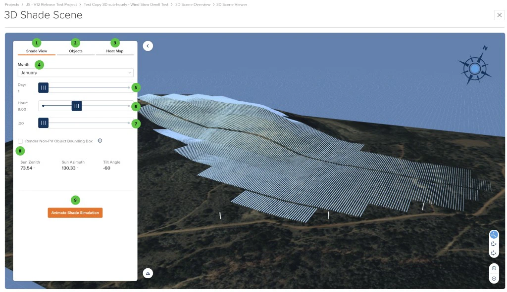
User Inputs (Shade View)
| # | Input | Type | Units | Description | Related Documentation |
|---|---|---|---|---|---|
| 1 | Shade View (Tab) | Tab | — | Currently selected tab. Provides real-time shading visualization for any timestamp in the weather file. The 3D scene shows shadows cast on PV surfaces based on sun position. | — |
| 2 | Objects (Tab) | Tab | — | Navigate to the Objects tab to add, edit, and manage shading objects within the 3D scene. | — |
| 3 | Heat Map (Tab) | Tab | — | Navigate to the Heat Map tab to visualize calculated shading results. Only available after 3D calculations have been completed on the 3D Scene Overview page. | 3D Scene Overview |
| 4 | Month | Dropdown | — | Select the month for the shading simulation. Combined with Day and Hour to define the specific timestamp for visualization. | — |
| 5 | Day | Slider | — | Select the day of the month using the slider or play button. The play button animates through all days of the selected month to show seasonal shading progression. | — |
| 6 | Hour | Slider | — | Select the hour of the day using the slider or play button. The play button animates through all hours to show daily shadow movement from sunrise to sunset. | — |
| 7 | Minutes | Slider | — | Select the minute interval within the selected hour. This control is only visible when the associated weather file uses sub-hourly time resolution (e.g., 15-minute or 5-minute intervals). | — |
| 8 | Sun Position & Tilt | Read-only | ° | Displays the current Sun Zenith, Sun Azimuth, and Tilt Angle for the selected timestamp. These values update dynamically as time controls are adjusted. | — |
| 9 | Animate Shade Simulation | Button | — | Starts an animated visualization cycling through timestamps to show shadow patterns across the selected time period. Useful for understanding overall shading behavior. | — |
Objects
The Objects tab provides tools for adding and managing shading objects directly within the 3D scene. Users can create walls, polygons, and cylinders to represent nearby structures, vegetation, or other obstructions that cast shadows on the PV array. For georeferenced scenes, satellite and terrain imagery is overlaid on the 3D surface, and the terrain buffer can be adjusted to extend imagery beyond the layout bounds.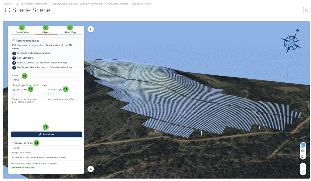
User Inputs (Objects)
| # | Input | Type | Units | Description | Related Documentation |
|---|---|---|---|---|---|
| 10 | Shape | Dropdown | — | Select the type of shading object to create. Options include: Wall (straight runs such as fences, walls, or barriers — requires Width and Height), Polygon (enclosed area such as a building footprint — requires Height), and Cylinder (round object such as a pole or tree trunk — requires Radius and Height). | — |
| 11 | Width (W) | Numeric | m / ft | Thickness of the shading object along the ground, perpendicular to the line. Applicable to the Wall shape type. Units depend on the project’s units toggle setting. | — |
| 12 | Height (H) | Numeric | m / ft | Height of the shading object above the terrain surface. Applicable to Wall, Polygon, and Cylinder shape types. Units depend on the project’s units toggle setting. | — |
| 13 | Start Draw | Button | — | Begins the interactive drawing mode in the 3D viewer. For a Cylinder, single-click on the terrain to place the object. For a Wall or Polygon, single-click to place each vertex and double-click to complete the shape. After drawing, use Save or Discard at the top of the view to confirm or cancel. | — |
| 14 | Terrain Buffer | Numeric | m / ft | Extends the satellite and terrain surface imagery beyond the bounds of the layout by the specified distance. A larger buffer provides more visible ground context around the PV arrays in the 3D view. Only applicable to georeferenced scenes where satellite/terrain imagery is available. Units depend on the project’s units toggle setting. | — |
Heat Map
The Heat Map tab displays calculated shading results as color-coded heat maps overlaid on PV surfaces. Four different metrics can be visualized, each showing DNI-weighted annual results. The color scale can be toggled between Absolute and Relative modes.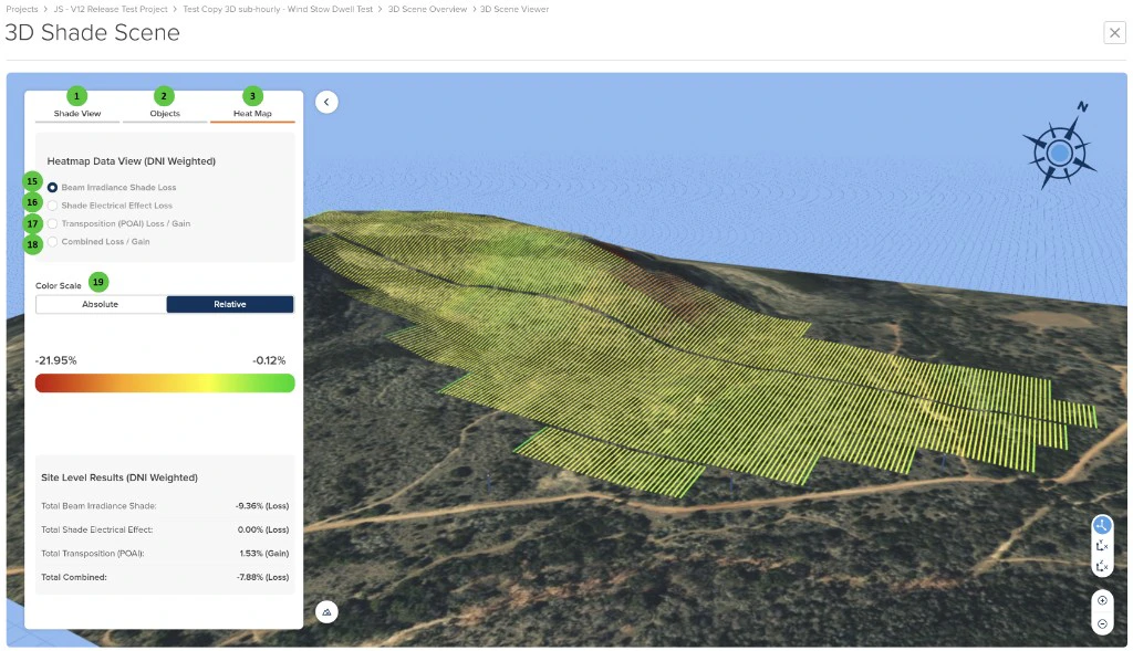
User Inputs (Heat Map)
| # | Input | Type | Units | Description | Related Documentation |
|---|---|---|---|---|---|
| 15 | Beam Irradiance Shade Loss | Radio Button | — | Display heat map showing direct/beam irradiance losses due to shading. Red indicates higher losses, green indicates lower losses. | 3D Shading |
| 16 | Shade Electrical Effect Loss | Radio Button | — | Display heat map showing non-linear electrical losses due to partial shading on module strings. Accounts for bypass diode activation and mismatch effects. | Electrical Shading |
| 17 | Transposition (POAI) Loss / Gain | Radio Button | — | Display heat map showing plane-of-array irradiance transposition effects. Values can be positive (gain) or negative (loss) relative to the reference calculation. Accounts for diffuse and reflected irradiance components. | Transposition Models |
| 18 | Combined Loss / Gain | Radio Button | — | Display heat map showing the net combined effect of all three factors: beam shade loss, electrical effect loss, and transposition loss/gain. | — |
| 19 | Color Scale | Toggle | — | Toggle between Absolute and Relative color scaling. Absolute uses a fixed scale across all surfaces; Relative scales colors to the min/max values of the current view, providing better contrast for subtle variations. | — |
- Total Beam Irradiance Shade — Site-wide beam shading loss percentage
- Total Shade Electrical Effect — Site-wide non-linear electrical loss percentage
- Total Transposition (POAI) — Site-wide transposition gain or loss percentage
- Total Combined — Net combined effect of all shading factors